Other posts
#
Branch Prediction
13 Jan
#processor design
#cache
#book
2024
I have always been passionate about how the CPU (Central Processing Unit, aka processor) works internally. However, the state-of-the-art knowledge of how the CPU works internally is a well-guarded secret. Each of the well-known CPU brands, like Intel, AMD, and recently Apple, has some secret sauce, or internal implementation, to be precise, of how it all works internally. It is not “just a CPU”; multiple independent units form a CPU. These independent units are, for example, cache, buses, branch prediction unit, data flow prediction, register array, execution unit, fetching unit, decoding unit, and many more!
For the programmer, how the CPU operates internally is often not crucial because the CPU exposes a certain API, and that is how the programmer can interact with it. The programmer, in most of the cases, does not need to know how the pipelining, out-of-order execution, data flow optimization, or other prediction work to make the application work correctly. It is the CPU’s work to execute the instructions correctly. The programmer’s responsibility is just to uphold the API of the CPU (or architecture, to be specific) so the CPU can make correct assumptions.
I stumbled upon a really great book, Modern Processor Design, by John Paul Shen and Mikko H. Lipasti. And it summarizes all the secret sauce that was implemented into the processors around the 00s. Yes, it is over 20 years old (as of the day of the writing this), and current CPU “implementations” will definitely include better algorithms, but we can take a glimpse of how the CPU designers were thinking back in the day. But keep in mind that we can only speculate whether the mentioned algorithms are still present or were replaced by something else, but still, they lay down the necessary foundations.
## What is branch prediction?
Branch prediction is an optimization technique that can speed up instruction execution. CPU on the input has a sequence of instructions, where the CPU iterates over them one by one. Now imagine code that contains branching (if statements); in this case, the CPU execution must continue only in the branch that was taken. Branch prediction tries to predict in which direction the code execution will continue without even executing that instruction! This technique is necessary in pipelined CPUs.
The following algorithms only make use of the address of the current branch and other information that is immediately available. Modern processors use a multi-cycle pipelined instruction cache, and therefore, the prediction for the next instruction must be available several cycles before the current instruction is fetched.
## Static Prediction
Static prediction techniques are used during the compilation of the program. After the program is compiled, the prediction hints are set in stone and cannot be modified without recompiling. Overall, they rely on compiler reordering of the code to speed up the execution of the program.
### Single Direction Prediction
When branching occurs, always take the branch (make the jump). It has the nice feature of not requiring modification to the Instruction Set Architecture (ISA), so it does not require special instruction to prefer a specific branch over another.
### Ball & Larus Heuristic
Some instruction set architectures provide an interface via the compiler through which the branch prediction hints can be made. For example, the following code:
| |
It will almost always succeed with memory allocation1. Thus, it makes sense to hint to the compiler that the handleError() branch is unlikely. Based on the previous assumption, Bell & Larus found out that with the following branch prediction rules, we can speed up the execution of the program.
| Heuristic name | description |
|---|---|
| Loop branch | If the branch target is back to the head of a loop, predict taken. |
| Pointer | If a branch compares a pointer with NULL, or if two pointers are compared, predict in the direction that corresponds to the pointer being not NULL, or the two pointers not being equal. |
| Opcode | If a branch is testing that an integer is less than zero, less than or equal to zero, or equal to a constant, predict in the direction that corresponds to the test evaluating to false. |
| Guard | If the operand of the branch instruction is a register that gets used before being redefined in the successor block, predict that the branch goes to the successor block. |
| Loop exit | If a branch occurs inside a loop, and neither of the targets is the loop head, then predict that the branch does not go to the successor that is the loop exit. |
| Loop header | Predict that the successor block of a branch that is a loop header or a loop preheader is taken. |
| Call | If a successor block contains a subroutine call, predict that the branch goes to that successor block. |
| Store | If a successor block contains a store instruction, predict that the branch does not go to that successor block. |
| Return | If a successor block contains a return from subroutine instruction, predict that the branch does not go to that successor block. |
### Profiling Technique
It involves compiling code with special probes that collect statistics, followed by executing test runs with input sample data. Based on the results of these test executions, the compiler hints will be generated. However, the branch hints will be set in stone, and further modification of them will require binary recompilation.
## Dynamic Prediction
The main idea behind dynamic algorithms is to use the outcome of the branch execution to determine the outcome of the subsequent execution of the same branch. This means when the branch was taken, it will probably be retaken next time.
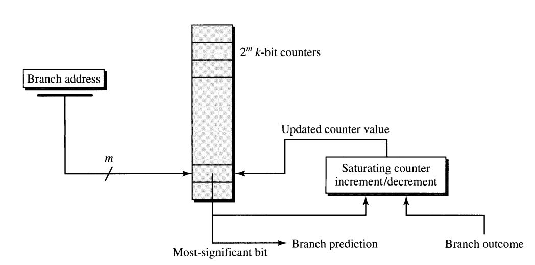
### Smith’s Algorithm
The main idea is to have $2^m$ counters, where each counter keeps the outcome of the branching, where the counter is incremented if the branch was taken and decremented if it was not taken. Since we have only a limited amount of counters, often much lower than the number of possible addresses that can be stored in the Program Counter (PC), we need to hash down the address from the PC to $m$ bits, where each counter has a defined width of $k$ bits. Hint is based on the most significant bit of the counter. The counter is often 2-bit wide, so if we have only true branches followed by one false branch. The branch prediction will still recommend the true branch even though the last branch was false; this effect is called hysteresis.
Modem implementations use a simple PC mod $2^m$ hashing function.
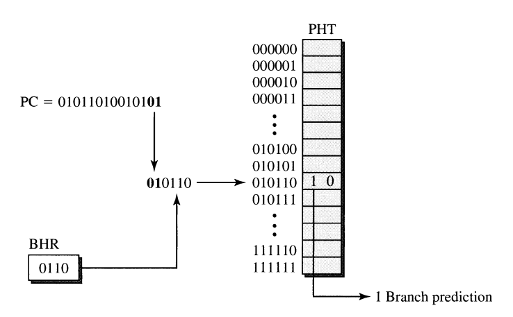
### Two-level Prediction Tables
Employs two separate levels of branch history to make the branch prediction. It is effectively an extension of the Smith’s Algorithm.
However, in this case, the terminology expands to cover more cases. Let’s call the array of counters Pattern History Table (PHT). We can modify or increase the number of input values to get better hashing results. In the previous case, it hashed only the PC. But what is stopping us from including more variables in the hashing function?
To increase entropy, we can include a Branch History Register (BHR) in the hashing function. BHR is a shift register that contains outcomes of the most recent branch outcomes2.
The key to the PHT can be constructed from ANY path, so there can be conflicts (or cache key collisions, to be precise). There can be multiple sources whose path can point to the particular PHT entry, where each source can result in a different outcome of the branching point.
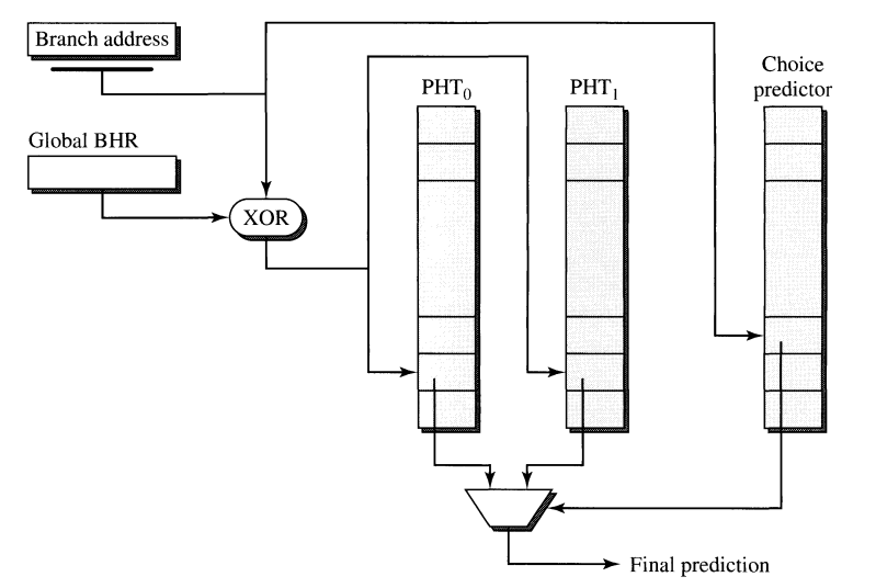
### Bi-Mode Predictor
Bi-Mode predictor has this multilayer fashion, where we have two PHTs, and the PHT selector selects the correct PHT. The PHT selector has the branch address from the PC, and based on that, it decides which PHT will be used for prediction.
## Hybrid Prediction
Hybrid predictors integrate the heuristics of both dynamic and static predictors. In practical terms, heuristics with a greater number of “input variables” tend to produce better outcomes. A larger available context allows us to leverage additional information for improved prediction accuracy.
### Tournament Predictor
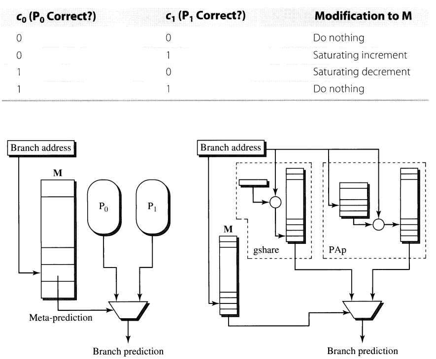
Tournament predictor consists of two predictors $P_i$, where $i \in \{0, 1\}$ and meta predictor $M$.
The $P_i$ can be any of the static or dynamic predictors that were mentioned earlier, and The $M$ is basically a table that stores the outcomes.
We can think of this predictor as the actual tournament (as the name suggests), where there are two fighters where each of them competes. However, the real fighters are the results from the $P_i$; the responsibility of the referee is to combine the outputs from the $P_i$ and decide on the final value. The output verdict of the referee is either to increase the value in the PMT or decrease the value in the PMT.
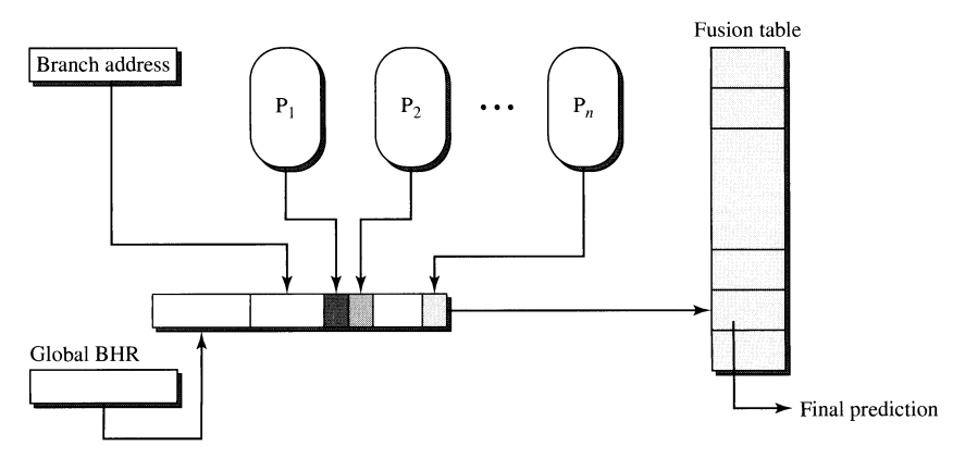
### Prediction fusion
Predictor fusion combines results from $P_0, P_1,\dots, P_n$ into making a final prediction. Again, it shares the same principles as the previous ones, but in this case, we are not limited to a limited number of predictors. It is also based on the hashing function that has $n$ variables on the output, and the result of the hashing function is an index into the Fusion table (or PMT, if we would like to share the same terminology).
The specific method of how the key into the Fusion table is constructed is implementation dependent.